Most charts use some kind of a legend to help readers understand the charted data. Whenever you create a chart in Excel, a legend for the chart is automatically generated at the same time. A chart can be missing a legend if it has been manually removed from the chart, but you can retrieve the missing legend.
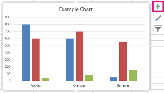
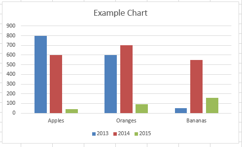
This example chart shows a legend explaining the colors for the years 2013, 2014, 2015.
In this article

Add a chart legend
-
Select the chart.
-
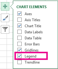
Select Chart Elements
-
Select the Legend check box.
The chart now has a visible legend.
Edit legend texts
If the legend names in the chart are incorrect, you can rename the legend entries.
-
Select the chart.
-
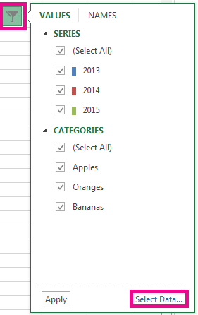
Select Chart Filters
-
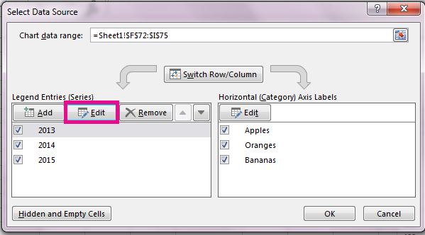
Select an entry in the Legend Entries (Series) list and select Edit.
-
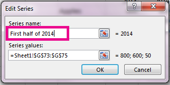
In the Series Name field, type a new legend entry.
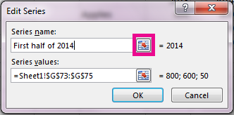
Tip: You can also select a cell from which the text is retrieved. Select the Identify Cell button
-
Select OK.


